The recording
You were last reading slide 1.
Search systems
FAISS, Elasticsearch and deep research
Information Retrieval for AI
Monday 12 October 2026
KAIST AI - Seong Joon Oh
Announcements
Wednesday 14 October: guided paper-search workshop
14 October, 09:00-10:00 KST, on Zoom.
Open the workshop and follow the lecturer with the supplied starter. Access and the baseline run take place in class.
The workshop carries 2 project marks. Today’s vector DB and chunking material prepares the comparison.
Next week: LIMIT discussion
Wednesday 21 October, 09:00-10:00 KST, on Zoom.
LIMIT: On the Theoretical Limitations of Embedding-Based Retrieval
Read the anchor and the relevant sections of one supporting paper you choose. Preparation is due Tuesday 20 October at 18:00 KST.
Roadmap
FAISS
Facebook AI Similarity Search
Efficient nearest-neighbour search
Exact search, inverted files, graph search and product quantisation.
FAISS makes vector search practical
Coarse retrieval needs the nearest document vectors for a query. We already have embeddings and a similarity score. The problem is how to find the top matches efficiently as the corpus grows.
The cost: an exact scan scores every document vector for every query. Storing all full-precision vectors also consumes memory.
FAISS provides vector indexes with different trade-offs:
- Exact search: efficient implementations on CPUs and GPUs.
- IVF and HNSW: search selected lists or graph neighbours to reduce comparisons, with possible missed neighbours.
- PQ: compress vectors into short codes to reduce storage, with approximate scores.
Choose an index and tune it for the required speed, memory and neighbour recall.
Exact search is the reference
Each input row is a passage or query embedding. embedding_dim is its number of coordinates.
def exact_search(
    passage_embeddings,  # shape: (num_passages, embedding_dim)
    query_embeddings,    # shape: (num_queries, embedding_dim)
    top_k,               # number of hits per query
):
    """Return (similarity_scores, passage_rows), each (num_queries, top_k).

    similarity_scores: inner products, highest first.
    passage_rows: row indices into passage_embeddings.
    """
    embedding_dim = passage_embeddings.shape[1]
    exact_index = faiss.IndexFlatIP(embedding_dim)
    exact_index.add(passage_embeddings)
    similarity_scores, passage_rows = exact_index.search(
        query_embeddings, top_k
    )
    return similarity_scores, passage_rows
exact_index scans every stored vector. Its returned neighbours define the reference for ANN recall, not relevance labels.
Inverted file (IVF) search selects partitions
Build
- Embed each document or passage.
- Compute centroids with k-means on a representative sample. Repeatedly assign vectors to the nearest centroid, then recompute centroids as cluster means.
- Assign every corpus vector to its nearest centroid. Store its vector and document ID in that centroid’s inverted list.
More probes scan more lists: higher search cost, fewer missed neighbours.
HNSW: building
Hierarchical navigable small world (HNSW). Each node is a document vector; each edge is a stored link.
- Route: C belongs to layers 1 and 0. Search layer 2 for a starting point.
- Connect: in layer 1, follow existing links to find nearby candidates. Select neighbours, add links both ways, and prune excess links.
- Repeat: use the candidates found to start the same process in layer 0.
M controls connectivity; efConstruction controls how broadly insertion searches for candidates.
HNSW: processing query
- Top: start in layer 2. Follow stored links to vectors closer to the query.
- Descend: when no linked neighbour is closer, move down at the same vector. Repeat in layer 1, then descend to layer 0.
- Bottom: explore several paths through the links. Keep up to
efSearchbest vectors found.
Stop when no pending candidates remain, or the closest pending candidate is farther than the worst retained result. Return the best
Larger efSearch allows more exploration at greater cost. It limits retained results, not total visits; the answer remains approximate.
Product quantisation (PQ): building
Split the same coordinates in every document. For each group, compute 256 centroids with k-means across documents. These form a shared codebook for that group.
Store the document as [17, 203, 6, 91]. Each index selects a centroid from its own codebook.
Toy example:
PQ: processing query
Keep the query pieces uncompressed. The tables contain query-to-centroid dot products. Compute them when the query arrives; reuse them across documents.
Each document needs four lookups and a sum. Documents with the same centroid index reuse the same table entry. The result approximates the original dot product.
IndexPQ scans all codes; IndexIVFPQ scans codes in selected lists. Approximation can change neighbour order.
Which index fits the workload?
| Method | Storage | Per-query computation | Search accuracy |
|---|---|---|---|
| Exact | Medium | Heavy | Exact neighbours |
| IVF | Medium | Medium | Can miss neighbours in skipped lists |
| HNSW | Heavy | Light | Can miss neighbours outside explored paths |
| PQ | Light | Medium | Approximate scores can change neighbour order |
Search accuracy means agreement with exact vector search, not relevance to the query.
Typical guide for a large corpus. Hardware and recall settings can change these ratings; PQ saves memory but does not guarantee faster queries.
Connect each method to one context. Select a method, then a context. One point per correct match; submit once.
Your connections
Sign in with your course account to submit.
Elasticsearch
From a vector index to a search service
Chunk documents, index passages and retrieve evidence.
ElasticSearch: From nearest neighbours to a search service
We can now find nearby document vectors efficiently. What must happen around that search to serve a user?
“Find passages about battery recycling in papers published since 2024.”
- Chunk and store documents: split documents into passages; keep each chunk’s text, embedding, publication date and source link together.
- Retrieve candidates: match query words with BM25 and meaning with vector search.
- Apply constraints: restrict results to eligible publication dates.
- Operate the service: accept requests, update documents and distribute the index across machines.
Elasticsearch provides these capabilities through a search API. We will follow one passage record through keyword search, vector search and filters.
Its vector search uses Apache Lucene’s HNSW implementation. The graph-search principles we have studied still apply.
Chunking defines what we retrieve
A chunk is the text unit we index, embed and return. Its boundaries determine which context stays together.
| Strategy | Split at | Benefit | Limitation |
|---|---|---|---|
| Sentence | Sentence boundaries | Keeps sentences intact | Related sentences may separate |
| Word | A word-count limit | Controls chunk length | May cut a sentence in half |
| Recursive | Ordered separators, then finer boundaries | Follows document structure | Needs suitable separators |
| None | No additional split | Retains input or external chunks | Input must fit the model limit |
Boundary example: “Our battery recycling process recovered lithium. These results apply only to sorted cells.” Keep both sentences in Chunk A so the claim retains its qualification.
Size trades focused matches against context. Overlap can retain context across boundaries, but duplicates text and adds indexing work. Test both against retrieval examples and the embedding model’s input limit.
Adapted from Elastic’s chunking strategies.
Index each chunk with its source
Our example stores one Elasticsearch record per chunk. Compute its embedding with the same model used for queries.
Text, vector and metadata describe the same passage ID. A hit can return the passage text and source location; the document ID groups passages from the same paper.
Follow the query to its passages
Constructed candidates and rankings, not measured results. A is the chunk from paper 17; B and D are passages from other papers.
Deep Research
From search results to an evidence-based report
An agent chooses queries, checks evidence and writes the answer.
From search results to deep research
We can retrieve documents for a query. Who chooses the next query, decides whether the evidence is sufficient, and writes the answer?
Recall the laptop task: A PhD student needs a laptop for daily travel and large-dataset analysis: budget ₩2 million, weight at most 1.5 kg, RAM at least 32 GB. Compare three models sold in Korea, recommend one and cite the evidence.
Interactive search: search → results → a human checks evidence and directs the next search.
Deep research: search → results → an agent checks evidence and chooses further searches → report.
The user sets the objective. The agent uses search systems within a multi-step investigation. Human attention need not direct every search round.
A cheap 16 GB listing does not establish the price of the exact 32 GB configuration. The agent must find and check that missing evidence.
Constructed task from our earlier example. Anthropic’s research-system account, 2025
What should the investigation achieve?
Laptop task: Compare three models sold in Korea and recommend one within the stated budget, weight and RAM requirements.
- Correctness and support: Verify each claim against the exact configuration and its cited source.
- Breadth and depth: Cover the requested alternatives and criteria; explain the trade-offs and unresolved evidence.
- Efficiency: Count elapsed time, tokens, tool calls and cost across the entire campaign.
A relevant result list is an intermediate output. Evaluate the final answer or report, then inspect the trace to explain failures.
Compare quality at a fixed budget, or cost at a stated quality target. State the source environment and judge.
Benchmarks test different outputs
| Name | What’s measured | Data | Metric |
|---|---|---|---|
| BrowseComp | Find a hard-to-locate answer | Human-authored web questions with short reference answers | Answer accuracy |
| BrowseComp-Plus | Answer and evidence retrieval | BrowseComp-derived questions; fixed web corpus and evidence labels | Answer accuracy; evidence recall; retriever nDCG |
| DeepSearchQA | Return a complete, correct answer set | Multi-step web questions with reference answer sets | Answer-set precision, recall and F1 |
| DeepResearch Bench | Report quality and citation support | Expert-written research tasks and reference reports | RACE report score; FACT citation accuracy and effective citation count |
Record time, tokens and tool cost beside quality. The tasks and judges differ; their scores are not interchangeable.
How to build a deep-research system
Request → research brief → model chooses an action → harness executes a tool → model reads the observation → further research → report.
Model: Proposes queries, source inspections and conclusions from the available evidence.
Harness: Runs tools, routes work, retains state and enforces limits.
Workflow: Connects clarification, research and report generation. It specifies where evidence and output checks occur.
Compare Anthropic’s published architecture with an open research model and source code for a report-producing harness.
Anthropic’s research system
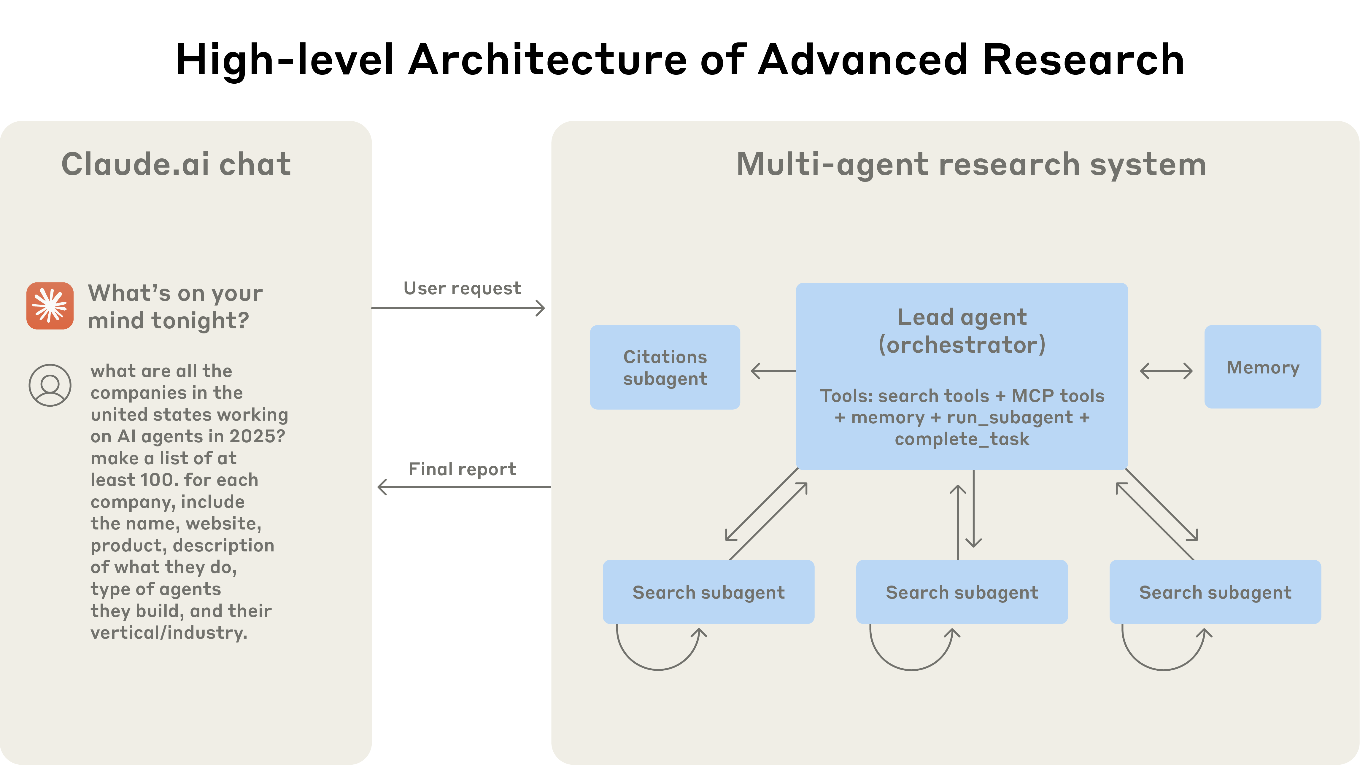
The lead researcher plans the investigation and delegates branches to workers with separate contexts. It combines their findings; a citation stage attaches sources.
For laptops, give each worker one candidate and the same requirements. The lead must reconcile configuration differences before comparison.
Parallel work adds breadth and token cost. This is the architecture described in June 2025.
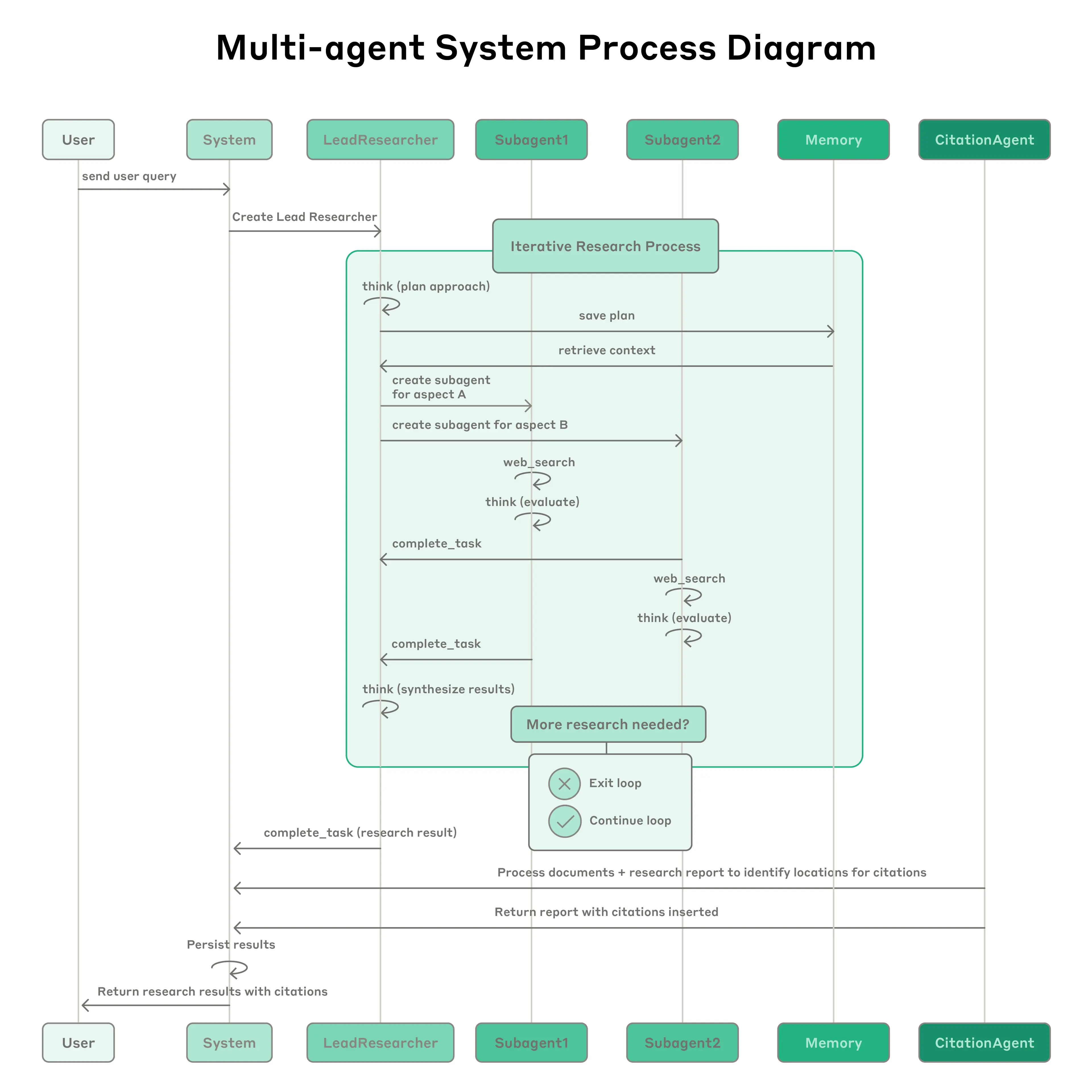
From a system description to open-source code
We now move from Anthropic’s published architecture to an implementation we can inspect.
Which implementation? LangChain’s Open Deep Research, a Python research workflow built with LangGraph. It connects language models and search tools to turn a user request into a research report. We inspect revision 1b7d2e80 of the archived repository.
Goal of the dissection: Trace how the laptop request becomes a report, and locate the code that controls quality and cost.
- Workflow and state: How does the request become a brief, and what information reaches each stage?
- Delegation and tools: How are workers launched, what do they receive, and how do their results return?
- Evidence and stopping: What survives compression, when does research stop, and what reaches the writer?
Open Deep Research: the complete workflow
The supervisor reappears at the decision point. Stop triggers: completion signal, no tool call, or iteration limit.
From research brief to report
- Brief and supervisor: turn the request into a shared brief. The supervisor assigns topics and reviews workers’ summaries.
- Parallel workers: each agent searches and reads with its own tools and conversation. The harness limits concurrent tasks; workers return summaries and raw notes.
- Stop and write: the supervisor can request more research. A completion signal, no tool call or an iteration limit ends the loop. The writer receives the brief and collected summaries; raw notes stay separate.
Preserve the evidence through each hand-off. For the laptop task, retain the ₩2 million budget, 1.5 kg weight limit and 32 GB requirement. A summary that drops “16 GB” from a low-price listing may support the wrong recommendation. Reaching a stopping condition does not guarantee complete evidence.
Brief and supervisor - Workers and returned results - Stopping rules - Compression and writer
How can we improve deep research?
The agent can make a poor decision, the workflow can lose evidence, or search can miss it. Each calls for a different improvement.
| Direction | What we change | Prior work and its evidence |
|---|---|---|
| Model training | Clarification, queries and tool use. For the laptop task, ask about an unstated RAM requirement. | Search-R1 improved search-assisted QA, not established long-report quality. IntentRL improved clarification and research performance with simulated users. |
| Harness design | Delegation, tool instructions and evidence hand-offs. Keep the configuration beside each price through compression. | Anthropic reports shorter completion times after tool-description improvements and parallel agent/tool execution in its research system. |
| Retrieval system | Sources, matching, context and reranking. Retrieve the Korean listing for the exact laptop configuration. | Contextual Retrieval reduced retrieval failures with contextualised chunks, BM25 plus embeddings, and reranking. It measured RAG retrieval recall, not research-report quality. |
Test whether a change improves supported report quality at the same cost, or reduces cost at the same quality. Test components separately before combinations.
Coming up
Wednesday 14 October - paper-search workshop
09:00-10:00 KST, on Zoom.
A guided, hands-on session with a paper-search system. Explore how retrieval choices affect its results.
Next Wednesday 21 October - LIMIT discussion
09:00-10:00 KST, on Zoom.
LIMIT: On the Theoretical Limitations of Embedding-Based Retrieval
Read the anchor paper and the relevant sections of one supporting paper. Preparation is due Tuesday 20 October at 18:00 KST.